The Histogram represents the distribution of the numeric data. A histogram is an estimate of the probability distribution of a continuous variable. It differs from a bar graph. The bar graph is related to the categorical variable, whereas the histogram is related to the numeric feature. A histogram is widely used in the data analysis task. This tutorial has demonstrated a various method to plot histogram.
A pyplot.hist() method used to plot a histogram of numeric data points.
Parameters :
- x : Input values
- bins : no of bins
- range : the lower and upper range of the bins.
- density : bool
- weight : An array of weights, of the same shape as x.
- bottom : Location of the bottom baseline of each bin
- align : {‘left’, ‘mid’, ‘right’}, optional
- orientation : {‘horizontal’, ‘vertical’}, optional
- label : label of the histogram
- color : color of the histogram
Example:
import matplotlib.pyplot as plt
import numpy as np
from matplotlib import colors
from matplotlib.ticker import PercentFormatter
N_points = 100000
n_bins = 20
x = np.random.randn(N_points)
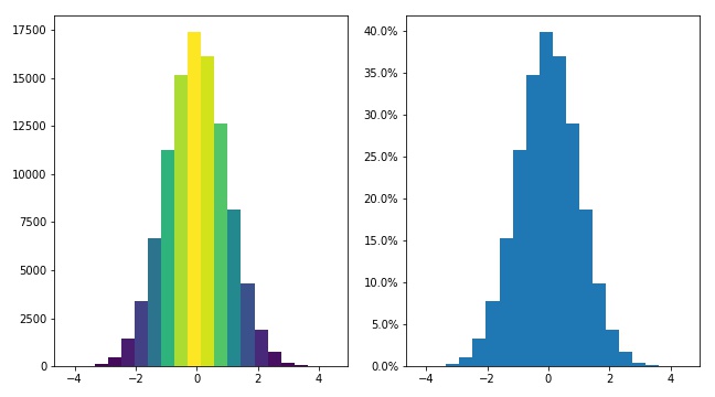
fig, axs = plt.subplots(1, 2, figsize=(9,5),tight_layout=True)
# N is the count in each bin, bins is the lower-limit of the bin
N, bins, patches = axs[0].hist(x, bins=n_bins)
# We'll color code by height, but you could use any scalar
fracs = N / N.max()
# we need to normalize the data to 0..1 for the full range of the colormap
norm = colors.Normalize(fracs.min(), fracs.max())
# Now, we'll loop through our objects and set the color of each accordingly
for thisfrac, thispatch in zip(fracs, patches):
color = plt.cm.viridis(norm(thisfrac))
thispatch.set_facecolor(color)
# We can also normalize our inputs by the total number of counts
axs[1].hist(x, bins=n_bins, density=True)
# Now we format the y-axis to display percentage
axs[1].yaxis.set_major_formatter(PercentFormatter(xmax=1))
plt.show()
This produces the following result:
. . .
import numpy as np
import matplotlib.mlab as mlab
import matplotlib.pyplot as plt

mu = 100 # mean of distribution
sigma = 15 # standard deviation of distribution
x = mu + sigma * np.random.randn(10000)
num_bins = 20

n, bins, patches = plt.hist(x, num_bins, normed=1, facecolor='green', alpha=0.5)
# add a 'best fit' line
y = mlab.normpdf(bins, mu, sigma)
plt.plot(bins, y, 'r-o')

plt.xlabel('X')
plt.ylabel('Probability')
plt.title(r'Histogram : $\mu=100$, $\sigma=15$')
# Tweak spacing to prevent clipping of ylabel
plt.subplots_adjust(left=0.15)
plt.show()

. . .