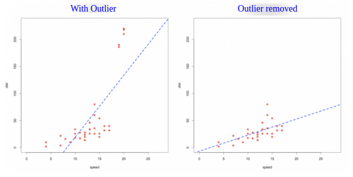
An outlier is an observation in the data, which is distant from other observation. To deal with outlier itself is a very challenging task in Machine Learning. Outlier generally exists in the data due to instrument error, human error or fraudulent behaviour. Here, I have explained the outlier detection techniques and how they impact on Machine Learning algorithms. And also, Explained different techniques to handle outliers in the data. Generally, Outlier is detected using graphic visualization.
Here, I have used the Kaggle’s data House Prices: Advanced Regression Techniques for demonstration. We need to predict house price from features of the house. There is one feature exist in the Data called LotArea. LotArea represents the Lot size in square feet.
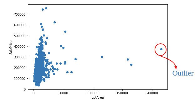
Let’s plot this feature using matplotlib library.

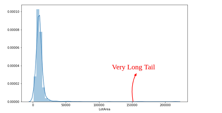
You can see the extreme value as an outlier in the plot. Outlier also visualize in the histogram of feature values, they may be the values on the tails.

Using the above graph, we can conclude that the feature LotArea (Lot size in square feet) contain outlier with 2,00,000 value.
We can also observe the outlier using Pandas’ Library.
train['LotArea'].describe()

This depicts the distribution of the feature values. 25th percentile is 7553, 50th percentile is 9478 and 75% percentile is 11601 and the maximum value is 215245.
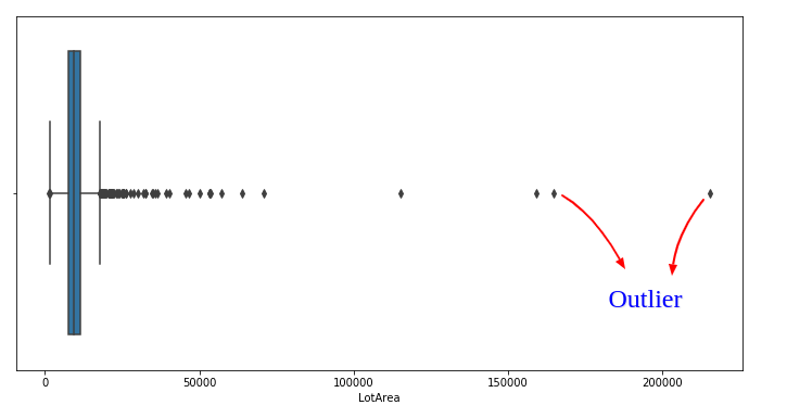
We can also Observe this distribution using Boxplot. Boxplot represents the distribution of the feature.

Let’s plot the Boxplot of feature LotArea.

Resolve outlier
It is not a good idea to drop Outlier from the data every time instead we should impute the outlier by most suitable value. We can safely remove the outlier if we are 99 per cent sure that it’s an error. If we drop the data, we lose information. Machine Learning model predicts abnormally with such outliers in the data.

Here, I have described the different methods to deal with an Outlier.
1) Winsorization:
Clip Feature values between lower bound and upper bound. We can choose these lower bound and upper bound values using the percentile of the feature. For Example, we can select 1st and 99th percentile as lower and upper bound values respectively. This method is called the Winsorization.

2) Rank Transformation
The rank transformation will move the outlier closer to other values. The Scipy Python library provides scipy.stats.rankdata function to apply the rank transformation.
from scipy.stats import rankdata
rankdata([-1000,0,2])       →  [1,2,3]
rankdata([1,5,2,50000])     →  [1,3,2,4]
3) Log Transformation
A Log transformation drives too big values closer to the feature’s mean values.
train['log_LotArea'] = np.log(1+train['LotArea'])
