Cosine Similarity – Text Similarity Metric

Text Similarity has to determine how the two text documents close to each other in terms of their context or meaning. There are various text similarity metric exist such as Cosine similarity, Euclidean distance and Jaccard Similarity. All these metrics have their own specification to measure the similarity between two queries.

In this tutorial, you will discover the Cosine similarity metric with example. You will also get to understand the mathematics behind the cosine similarity metric with example. Please refer to this tutorial to explore the Jaccard Similarity.

Cosine similarity is one of the metric to measure the text-similarity between two documents irrespective of their size in Natural language Processing. A word is represented into a vector form. The text documents are represented in n-dimensional vector space.

Mathematically, Cosine similarity metric measures the cosine of the angle between two n-dimensional vectors projected in a multi-dimensional space. The Cosine similarity of two documents will range from 0 to 1. If the Cosine similarity score is 1, it means two vectors have the same orientation. The value closer to 0 indicates that the two documents have less similarity.

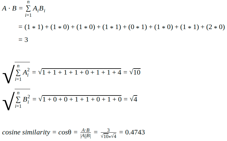
The mathematical equation of Cosine similarity between two non-zero vectors is:

Let’s see the example of how to calculate the cosine similarity between two text document.

doc_1 = "Data is the oil of the digital economy" 
doc_2 = "Data is a new oil" 

# Vector representation of the document
doc_1_vector = [1, 1, 1, 1, 0, 1, 1, 2]
doc_2_vector = [1, 0, 0, 1, 1, 0, 1, 0]

The Cosine Similarity is a better metric than Euclidean distance because if the two text document far apart by Euclidean distance, there are still chances that they are close to each other in terms of their context.

Compute Cosine Similarity in Python

Let’s compute the Cosine similarity between two text document and observe how it works.

The common way to compute the Cosine similarity is to first we need to count the word occurrence in each document. To count the word occurrence in each document, we can use CountVectorizer or TfidfVectorizer functions that are provided by Scikit-Learn library.

Please refer to this tutorial to explore more about CountVectorizer and TfidfVectorizer.

TfidfVectorizer is more powerful than CountVectorizer because of TF-IDF penalized the most occur word in the document and give less importance to those words.

Define the Data

Let’s define the sample text documents and apply CountVectorizer on it.

doc_1 = "Data is the oil of the digital economy"
doc_2 = "Data is a new oil"

data = [doc_1, doc_2]

Call CountVectorizer

from sklearn.feature_extraction.text import CountVectorizer

count_vectorizer = CountVectorizer()
vector_matrix = count_vectorizer.fit_transform(data)
vector_matrix

<2x8 sparse matrix of type '<class 'numpy.int64'>'
	with 11 stored elements in Compressed Sparse Row format>

The generated vector matrix is a sparse matrix, that is not printed here. Let’s convert it to numpy array and display it with the token word.

Here, is the unique tokens list found in the data.

tokens = count_vectorizer.get_feature_names()
tokens

['data', 'digital', 'economy', 'is', 'new', 'of', 'oil', 'the']

Convert sparse vector matrix to numpy array to visualize the vectorized data of doc_1 and doc_2.

vector_matrix.toarray()

array([[1, 1, 1, 1, 0, 1, 1, 2],
       [1, 0, 0, 1, 1, 0, 1, 0]])

Let’s create the pandas DataFrame to make a clear visualization of vectorize data along with tokens.

import pandas as pd

def create_dataframe(matrix, tokens):

    doc_names = [f'doc_{i+1}' for i, _ in enumerate(matrix)]
    df = pd.DataFrame(data=matrix, index=doc_names, columns=tokens)
    return(df)

create_dataframe(vector_matrix.toarray(),tokens)

       data  digital  economy  is  new  of  oil  the
doc_1     1        1        1   1    0   1    1    2
doc_2     1        0        0   1    1   0    1    0

Find Cosine Similarity

Scikit-Learn provides the function to calculate the Cosine similarity. Let’s compute the Cosine Similarity between doc_1 and doc_2.

from sklearn.metrics.pairwise import cosine_similarity

cosine_similarity_matrix = cosine_similarity(vector_matrix)
create_dataframe(cosine_similarity_matrix,['doc_1','doc_2'])

          doc_1     doc_2
doc_1  1.000000  0.474342
doc_2  0.474342  1.000000

By observing the above table, we can say that the Cosine Similarity between doc_1 and doc_2 is 0.47

Let’s check the cosine similarity with TfidfVectorizer, and see how it change over CountVectorizer.

Call TfidfVectorizer

from sklearn.feature_extraction.text import TfidfVectorizer

Tfidf_vect = TfidfVectorizer()
vector_matrix = Tfidf_vect.fit_transform(data)

tokens = Tfidf_vect.get_feature_names()
create_dataframe(vector_matrix.toarray(),tokens)

           data  digital  economy        is       new       of       oil      the
doc_1  0.243777  0.34262  0.34262  0.243777  0.000000  0.34262  0.243777  0.68524   
doc_2  0.448321  0.00000  0.00000  0.448321  0.630099  0.00000  0.448321  0.00000

cosine_similarity_matrix = cosine_similarity(vector_matrix)
create_dataframe(cosine_similarity_matrix,['doc_1','doc_2'])

          doc_1     doc_2
doc_1  1.000000  0.327871
doc_2  0.327871  1.000000

.     .     .