Machine Learning is the set of powerful mathematical operation. Machine Learning is built on mathematical principles like Linear Algebra, Calculus, Probability and Statistics. Basic understanding of mathematics is necessary to deeply understand machine learning phenomena. Here, I have described some essential foundation concepts of mathematics and the notations used to express them.
Vectors :
Vector is the central element of linear algebra. In the machine learning field, vector plays an important role while training models. Here, I have to explain the vector, how to define it using numpy and arithmetic operation on vectors.
Vector is a tuple of single or multiple values called scalars. Vector is representation in multi-dimension space.
Define a Vector
from numpy import array
arr1 = array([[10,25,15]])
arr2 = array([[10],[25],[15]])
print("shape of arr1 :",arr1.shape)
print("shape of arr2 :",arr2.shape)
Output:
shape of arr1 : (1, 3)
shape of arr2 : (3, 1)
Vector arithmetic operation:
Here, I have demonstrated arithmetic operation on vector where all operation is performed on the same size vector and generate the same size output vector.
Vector addition: addition of two vectors of the same size.
c = a + b
C[0] = a[0] + b[0]
C[1] = a[1] + b[1]
C[2] = a[2] + b[2]
from numpy import array
a = array([10,20,30])
b = array([10,20,30])
c = a+b
print(c)  #Output: [20 40 60]
Likewise vector addition, vector subtraction, multiplication and division operation are performed on the same sized vectors.
Vector Dot Product :
It’s also called the inner product of two vectors. The dot product is the sum of products of the corresponding entries of two vectors. This operation is widely used in machine learning.
Notation: c = a.b
The dot product of two vectors a = [a1, a2, …, an] and b = [b1, b2, …, bn] is defined as:
a.b = a1b1 + a2b2 + a3b3 + ……… + anbn
Numpy’s dot product np.dot function used for vector dot product.
import numpy as np
a = np.array([1,2,3])
b = np.array([1,2,3])
c = np.dot(a,b)
print(c)    #Output : 14
Linear function:
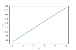
A linear function is a function whose graph is consist of a straight line throughout its domain. The main characteristic of a linear function is if the input variable is changed, the output variable is also changed proportionally to the input variable.
Let’s see linear function y = f(x) = 2x + 4
x = 0  →  f(x) = 4
x = 1  →  f(x) = 6
x = 2  →  f(x) = 8
x = 3  →  f(x) = 10
Here, x is called the variable.
Intercepts and Slope:
Slope-intercept is a prominent form of linear equations. It has the following general structure.
y = mx +b
Here, m and b can be any two real numbers. m is a slope and b is y-intercepts of y-coordinate.
For Example, the line y = 2x + 1 has a slope of 2 and a y-intercept at (0,1)

Quadratic Equations:
A Quadratic Equation is the equation of variable x and y has at least one variable with degree two.
Example: y = -2x2 + x + 3

Differential Calculus:

This linear function has the same gradient everywhere. Let’s pick two points in line and find the rate of changes using slope. The gradient of this line is equal to the amount of changes in vertical direction divided by the amount of changes in a horizontal direction. Using this equation, we can easily calculate the slope between two points. But, what is the slope at a single point in a line? In this case, this equation won’t work. The derivative will be used to find the slope at a single point in the graph.

This graph depicts the speed of the car at different timestamps. Here, the car’s speed is changing with respect to time. Initially, the speed of the car is zero at zero time and increasing with time which is also called accelerating. And at the end of time duration, car’s speed is rapidly decreasing which is called decelerating. This accelerating and decelerating is called the gradient of the speed-time graph. The gradient can be positive or negative. Acceleration has a positive gradient and deceleration has a negative gradient.
In this speed vs time graph, the gradient is different at every point. Let’s see how to calculate the gradient with examples.
Gradient at x = f’(x) = df/dx
Ex1.
f(x) = 3x + 2
Here, f(x) is the linear function. As per the above discussion, we know that the gradient of the linear function is constant. Let’s see the derivation of this function.
f’(x) = 3 It’s constant!
Ex2.
f(x) = x2
f’(x) = 2x

Let’s find the gradient at a point x = 0 and x = 1,
x = 0 → f’(0) = 2(0) = 0 (we can see that rate of change at point 0 is 0 in the graph)
x = 1 → f’(1) = 2(1) = 2
Multivariant Calculus:
Multivariate calculus is the extension of calculus with single variable functions to the calculus of multivariable functions. Multivariate calculus also is known as multivariable calculus.
Multivariant function:
A multivariant function is a function whose consists of multiple variables.
y = f(x,z) = 2x + 3z + 3
y = f(x,z) = 8x + 9z
These are the example of a multivariant function with a variable x and z.
How to find the derivative for changes in the multivariant function with respect to x and y?
Ans: Using Partial derivatives.
Partial derivatives :
The partial derivative of a multivariant function is its derivative with respect to one of those variable with other variable treated as constants.
Example.
z = f(x,y) = x2 + xy + y2
This is the partial derivative of function with respect to x. So, y is treated as constant.
∂f/∂x = 2x + y
This is the partial derivative of a function with respect to y. So, x is treated as constant.
∂f/∂y = 2y + x