Neural Network is a sophisticated architecture consist of a stack of layers and neurons in each layer. Neural Network is the mathematical functions which transfer input variables to the target variable and learn the patterns.
In this tutorial, you will get to know about the mathematical calculation that will happen behind the scene. To an outsider, a neural network may appear to be a magical black box but It has heavy mathematics calculation.
But, don’t worry. we don’t need to perform these mathematical calculations on the data. There are many deep learning libraries exist that work for you such as TensorFlow, Keras, PyTorch, etc.
However, it is necessary to understand the methodology, architecture and maths of the Neural Network. This tutorial will be helpful to learn the Neural Network in brief.
Neural network Architecture
Let’s define the architecture of the Neural Network. Here for the demonstration purpose, the 2-layer Neural Network is considered.
There are two input features x1 and x2 are fed into the input layer. A hidden layer has three neurons. Each neuron has assigned the weight parameter (w11, w12, w13, w21, w22, w23, w31, w41, w51) as shown in the below figure. Generally, these weight parameters are initialized randomly.
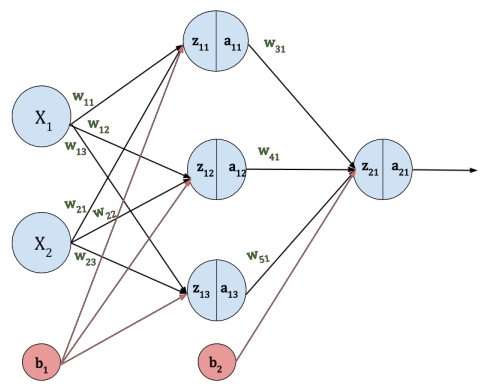
The b1 and b2 are the bias parameter for the input layer and hidden layer respectively. Neural Network is composed of the Forward propagation and Back-propagation. There are 5 steps of the Neural Network as follow:
- Initialize the weight & bias parameters
- Forward Propagation
- Compute the Loss
- Back-propagation
- Update the weight & bias parameters
Forward Propagation
In forward propagation, the input data are fed to the network in the forward direction. Each hidden layer gets the data, perform calculation and pass the result to the next layer. And Last, the output layer calculates the output of the model.
Let’s look at the mathematical equations of forward propagation. The z11, z12, z13 and z21 are the intermediate neuron value that is calculated from the weight, bias and neuron value of the previous layer.
An activation function will be applied to the intermediate neuron value to learn the non-linear patterns between inputs and target output variable. The a11, a12, a13 and a21 are the output of the activation function that is applied to the z11, z12, z13 and z21 respectively.
Below table represents the mathematical equations of the forward propagation and vector representation of it.
| Forward propagation equation | Vector Representation |
| z11 = x1 w11 + x2 w21 + b1 | 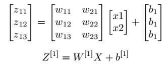 |
| z12 = x1 w12 + x2 w22 + b1 | |
| z13 = x1 w13 + x2 w23 + b1 | |
| a11 = σ (z11) |  |
| a12 = σ (z12) | |
| a13 = σ (z13) (σ – Activation function) | |
| z21 = a11 w31 + a12 w41 +a13 w51+ b2 |  |
| a21 = σ (z21) |  |
Compute the Loss (Error)

Back-Propagation Calculation
Backward propagation or backpropagation is the process of propagating the error(loss) back to the neural network and update the weights of each neuron subsequently by adjusting the weight and bias parameters.
Back-propagation plays an important role in the Neural Network. It performs several mathematical operations to learn the patterns between the input and the target variable.
The main goal of the neural network is to get the minimum error(loss). We can achieve a minimum error between an actual target value and predicted the target value if we get the correct value of the weight and bias parameters.
The error is change with respect to the parameters. This rate of change in error is to find by calculating partial derivation of the loss function with respect to each parameter.
By performing derivation, we can determine how sensitive is the loss function to each weight & bias parameters. This method is also known as Gradient Descent optimization method.
Let’s see how back-propagation work with an example. Here, we need to find the partial derivation of the loss function with respect to each parameter. Below section has described the calculations of the derivation.

In the above figure, the red line represents the back-propagation process. The da[2], dz[2], dw[2], db[2], da[1], dz[1], dw[1] and db[1] are the partial derivation of the loss function with respect to a[2], z[2], w[2], b[2], a[1], z[1], w[1] and b[1] respectively.
While performing the derivation calculation, we also need to calculate the derivation of the activation function. Let’s see the derivation of the Sigmoid Activation function.

Let’s see the calculation partial derivation of weight and bias parameters with respect to those parameters.


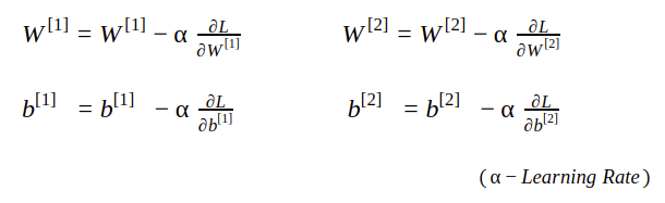
Weight Updating
The weight and bias parameters are updated by subtracting the partial derivation of the loss function with respect to those parameters.
Here α is the learning rate that represents the step size. It controls how much to update the parameter. The value of α is between 0 to 1.
If you want to understand more about the learning rate, please refer to this tutorial.
. . .