Learning Rate is one of the most important hyperparameter to tune for Neural network to achieve better performance. Learning Rate determines the step size at each training iteration while moving toward an optimum of a loss function. Generally, the Learning rate is denoted by the character α. The value of α is defined in the range between 0 and 1.
The direction towards an optimum of a loss function can be found by calculating the gradient of the loss function. The learning rate parameter specifies how big the step size is considered in that direction.
A Neural Network is consist of two procedure such as Forward propagation and Back-propagation.
- Forward propagation is also known as feedforward, which used to predict the output variable.
- Back-propagation method used to update the weight and bias of each layer to minimize the loss function.
In the Back-propagation method, the weight and bias parameters are updated using a gradient descent optimization algorithm. The Gradient descent optimization algorithm finds the gradient of the loss function.
The amount that the weights and bias parameters are updated is known as the learning rate. The mathematical equation to update the weight and bias parameters are as follow:

Here, the gradient term ?L/ ?W is the partial derivation of the loss function with respect to the weight parameter. That defines the rate of changes in the error with respect to the changes in the weight parameter.
While updating the weight parameters, it is better to use the fraction of gradient value instead of considering the full amount.
For example, if the learning rate is α = 0.1, means on each training iteration the weight parameters are updated only 10% of the gradient term.
Impact of Learning Rate on Neural Network
To find the optimal learning rate is a tedious task. The learning rate is a tuning parameter that controls the rate at which the model learns.
A too high learning rate allows the model to learn faster but, it might be overshooting the minimum point as the weight are updated rapidly.
A small learning rate allows the model to learn slowly and carefully. It makes the smaller changes to the weight on each update. hence takes too long to converge.
Learning rate that is too small may get stuck in an undesirable local minimum. Therefore, we should not use the learning rate too large and too small.
The learning rate value depends on your Neural Network architecture as well as your training dataset.
Find the Optimal Learning Rate
To achieve better performance of your neural network, it is necessary to find the optimal value of learning rate that is not too large and not too small. There are several approaches to find the best learning rate.
- Learning Rate Decay
- Learning Rate Schedule
- Adaptive Learning Rate
Learning Rate Decay
Learning rate is slowly reduces over each training epoch is referred to the Learning Rate Decay. Sometimes the fixed learning rate face difficulties to converge perhaps due to the noisy data or many other factors. Learning Rate Decay helps the model to converge at an optimal value.
It allows setting a large learning rate at the initial point and reduces it over time. This makes big changes to the weight update at the beginning of the training process and small changes towards the end of the training.
It is better to use the learning rate decay while training the neural network instead of using the fixed learning rate. However, the learning rate decay is another hyperparameter that you need to tune. The mathematical equation of learning rate decay is:

If the initial learning rate α0 = 0.2, then the learning rate at each epoch is :
|
Epoch |
Learning Rate |
| 1 | 0.198 |
| 2 | 0.194 |
| 3 | 0.188 |
| 4 | 0.180 |
| 5 | 0.171 |
Example of Learning Rate
Let’s develop the neural network on the iris dataset using Keras Deep learning library. you can set the fixed learning rate in Keras’ optimizer class. Let’s see how it work on iris data.
The learning rate is specified in Keras’ optimizer class. Below is the syntax to set learning rate 0.1 with stochastic gradient descent optimizer.
sgd = optimizers.SGD(lr=0.1)
model.compile(..., optimizer=sgd)
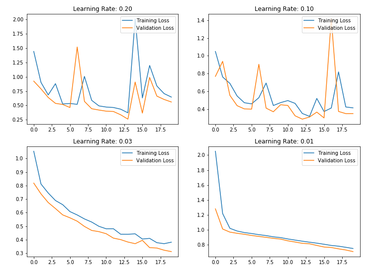
Let’s observe how our neural network works on iris data with different fixed learning rate.
# Import required packages
from tensorflow.keras.utils import to_categorical
from tensorflow.keras.models import Sequential
from tensorflow.keras.layers import Dense
from tensorflow.keras import optimizers
from sklearn.model_selection import train_test_split
import matplotlib.pyplot as plt
%matplotlib inline
from sklearn import datasets

# Load iris data
iris = datasets.load_iris()
X = iris.data
y = iris.target

Y = to_categorical(y)
X_train, X_test, y_train, y_test = train_test_split(X, Y, test_size=0.25, random_state=42)

# Define Neural Network model
def define_model():
    model = Sequential()
    model.add(Dense(50, input_dim=4, activation='relu'))
    model.add(Dense(12, activation='relu'))
    model.add(Dense(3, activation='softmax'))
    return model

# define Learning rates
l_r = [0.2,0.1,0.03,0.01]

plt.figure(figsize=(12,9))
for e in range(len(l_r)):
    sgd = optimizers.SGD(lr=l_r[e])

    model = define_model()
    model.compile(loss='categorical_crossentropy',optimizer=sgd, metrics=['accuracy'])
    history=model.fit(X_train, y_train,validation_data=(X_test,y_test), epochs=20, batch_size=32)

    _, accuracy = model.evaluate(X_test, y_test)
    print('Learning Rate: %f Test Accuracy: %.2f' % (l_r[e],accuracy*100))

    plt.subplot(2,2,e+1)
    plt.plot(history.history['loss'], label='Training Loss')
    plt.plot(history.history['val_loss'], label='Validation Loss')
    plt.legend(loc='upper right')
    plt.title('Learning Rate: %.2f' % (l_r[e]))
Example of Learning Rate Decay
The learning rate decay parameter can be specified in Keras’ optimizer class along with learning rate. Below is the syntax to set learning rate decay by defining the decay parameter with stochastic gradient descent optimizer class.
The default learning rate value is 0.01. And the learning rate decay parameter is set to 0 by default.
sgd = optimizers.SGD(lr=0.1,decay=0.01)
model.compile(..., optimizer=sgd)
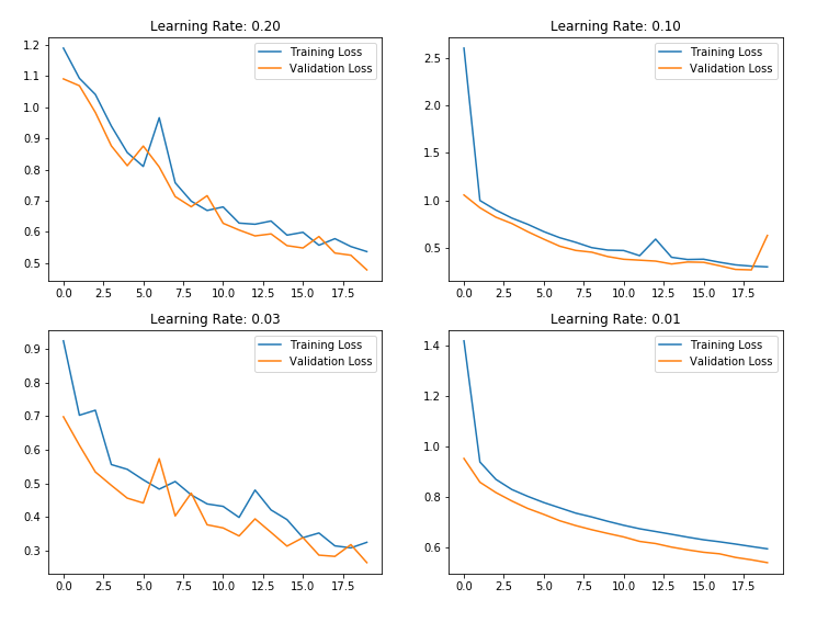
Let’s look at how our neural network work with learning rate decay while training the model instead of using the fixed learning rate.
# Import required packages
from tensorflow.keras.utils import to_categorical
from tensorflow.keras.models import Sequential
from tensorflow.keras.layers import Dense
from tensorflow.keras import optimizers
from sklearn.model_selection import train_test_split
import matplotlib.pyplot as plt
%matplotlib inline
from sklearn import datasets

# Load iris data
iris = datasets.load_iris()
X = iris.data
y = iris.target

Y = to_categorical(y)
X_train, X_test, y_train, y_test = train_test_split(X, Y, test_size=0.25, random_state=42)

# Define Neural Network model
def define_model():
    model = Sequential()
    model.add(Dense(50, input_dim=4, activation='relu'))
    model.add(Dense(12, activation='relu'))
    model.add(Dense(3, activation='softmax'))
    return model

# define Learning rates
l_r = [0.2,0.1,0.03,0.01]

plt.figure(figsize=(12,9))
for e in range(len(l_r)):
    sgd = optimizers.SGD(lr=l_r[e], decay=0.01)

    model = define_model()
    model.compile(loss='categorical_crossentropy',optimizer=sgd, metrics=['accuracy'])
    history=model.fit(X_train, y_train,validation_data=(X_test,y_test), epochs=20, batch_size=32)

    _, accuracy = model.evaluate(X_test, y_test)
    print('Learning Rate: %f Test Accuracy: %.2f' % (l_r[e],accuracy*100))

    plt.subplot(2,2,e+1)
    plt.plot(history.history['loss'], label='Training Loss')
    plt.plot(history.history['val_loss'], label='Validation Loss')
    plt.legend(loc='upper right')
    plt.title('Learning Rate: %.2f' % (l_r[e]))
. . .