Linear Regression is one of the famous algorithm in Machine Learning. Linear Regression model learns to understand the relationship between input variables and the output variable. The representation of Linear Regression is quite simple such, both input variables and output variable are numeric.
The linear regression uses a traditional slope-intercept equation where one scalar factor multiplies to each input variable called coefficient. And one additional coefficient is also added to the equation is called intercept or bias coefficient. There are mainly two types of Linear Regression:
Simple Regression
Simple Regression has a single input variable and a single output variable. For example, the equation of simple linear is like:
y = m*x + b
Here, x is an input variable and y is the output variable also our prediction.
Multivariable Regression
When we have more than a single input variable is called Multivariable Regression. A more complex Multivariable Regression equation looks like:
f(x,y,z) = w1x + w2y + w3z
Where, x,y,z represent the input variable and w1, w2, w3 represent the coefficient.
. . .
Example of Simple Regression
Let’s consider a dataset, which has a single called feature house area in square feet and need to predict the sale price of it.
| Area(Sq.ft) | Sale Price($) | |
| 1 | 500 | 100000 |
| 2 | 600 | 120000 |
| 3 | 800 | 150000 |
| 4 | 200 | 70000 |
| 5 | 350 | 78000 |
| 6 | 455 | 90000 |
| 7 | 560 | 110000 |
The simple linear regression equation will look like:
Sale Price = w1 * Area + b0
Here,
W1: The coefficient or weight for the Area independent variable.
Area: It is an input variable feature.
b0: The intercept where the line intercepts the y-axis. It is also known as bias.
Machine Learning algorithm will try to learn the correct values for weight and bias and approximate the line of best fit.
. . .
Cost function
The cost function finds the best optimize value for weight coefficients, which helps us to find the best fit line for data points. The cost function is the error rate between the observation’s target actual value and the predicted target value. The difference between the actual target value and the predicted target value is called error.
Let’s consider mean squared error(MSE) as a cost function. The MSE measured the averaged difference between the actual target values and predicted target values. The main goal is to minimize the error in order to improve the accuracy of the model.

Here, n is the number of observation.
. . .
Gradient descent
Gradient descent is a method of updating the weight coefficient iteratively in order to minimize the MSE by calculating the gradient of the cost function. Initially, random values are assigned to each coefficient.
Pred_y = mx+ b
Cost function  = (y - pred_y)2

Cost function :  f(m , b) = (y - (mx+b))2

df/dm = -2x (y - (mx + b))
df/db = -2 (y - (mx+b))
. . .
Learning Rate
The learning rate is the hyperparameter that controls the trained model on each iteration. It is the step size or scale factor which is considered while updating the weight and bias coefficient. Choosing an appropriate learning rate is also a challenging task as a too-small value may result in a long training process and large learning rate value has risk to overshoot the optimal point.
. . .
Model training with Linear Regression
Model training is the iterative procedure to improve the prediction by looping through the dataset multiple times. On each iteration, the weight and bias coefficient is updated using gradient descent. Model training is terminate when we get minimal error.
In [1]:
import numpy as np
import matplotlib.pyplot as plt
# generate random data-set
np.random.seed(0)
x = np.random.rand(100, 1)
y = 2 + 3 * x + np.random.rand(100, 1)
# plot the variable
plt.scatter(x,y)
plt.xlabel('x')
plt.ylabel('y')
plt.show()
Out[1]:
 In [2]:
def predict_sales(x, weight, bias):
return weight*x + bias
In [3]:
def cost_function(x, y, weight, bias):
data_size = len(x)
total_error = 0.0
for i in range(data_size):
total_error += (y[i] - (weight*x[i] + bias))**2
return total_error / data_size
In [4]:
def update_weights(x, y, weight, bias, learning_rate):
weight_deriv = 0
bias_deriv = 0
data_size = len(x)
for i in range(data_size):
# Calculate partial derivatives
# -2x(y - (mx + b))
weight_deriv += -2*x[i] * (y[i] - (weight*x[i] + bias))
# -2(y - (mx + b))
bias_deriv += -2*(y[i] - (weight*x[i] + bias))
# We subtract because the derivatives point in direction of steepest ascent
weight -= (weight_deriv / data_size) * learning_rate
bias -= (bias_deriv / data_size) * learning_rate
return weight, bias
In [5]:
def train(x, y, weight, bias, learning_rate, iters):
cost_history = []
for i in range(iters):
weight,bias = update_weights(x, y, weight, bias, learning_rate)
#Calculate cost for auditing purposes
cost = cost_function(x, y, weight, bias)
cost_history.append(cost)
# Log Progress
if i % 10 == 0:
print ("iter:{} weight:{} bias:{} cost:{}".format(i,weight,bias,cost))
return weight, bias, cost_history
In [6]:
weight, bias, cost_history = train(x, y, 0 ,0 ,0.1 ,50)
Out[6]:
iter:0 weight:[0.42198865] bias:[0.78929265] cost:[9.34952405]
iter:10 weight:[1.74059406] bias:[2.9879798] cost:[0.2134892]
iter:20 weight:[1.94959115] bias:[3.04804582] cost:[0.15774209]
iter:30 weight:[2.07759377] bias:[2.99278683] cost:[0.138376]
iter:40 weight:[2.18626937] bias:[2.93826919] cost:[0.12367039]
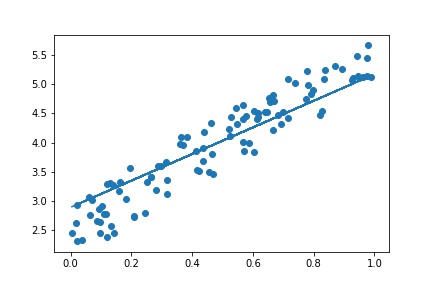
In [7]:
regression_line = [(weight*e)+bias for e in x]
plt.scatter(x,y)
plt.plot(x, regression_line)
plt.show()
Out[7]:
In [2]:
def predict_sales(x, weight, bias):
return weight*x + bias
In [3]:
def cost_function(x, y, weight, bias):
data_size = len(x)
total_error = 0.0
for i in range(data_size):
total_error += (y[i] - (weight*x[i] + bias))**2
return total_error / data_size
In [4]:
def update_weights(x, y, weight, bias, learning_rate):
weight_deriv = 0
bias_deriv = 0
data_size = len(x)
for i in range(data_size):
# Calculate partial derivatives
# -2x(y - (mx + b))
weight_deriv += -2*x[i] * (y[i] - (weight*x[i] + bias))
# -2(y - (mx + b))
bias_deriv += -2*(y[i] - (weight*x[i] + bias))
# We subtract because the derivatives point in direction of steepest ascent
weight -= (weight_deriv / data_size) * learning_rate
bias -= (bias_deriv / data_size) * learning_rate
return weight, bias
In [5]:
def train(x, y, weight, bias, learning_rate, iters):
cost_history = []
for i in range(iters):
weight,bias = update_weights(x, y, weight, bias, learning_rate)
#Calculate cost for auditing purposes
cost = cost_function(x, y, weight, bias)
cost_history.append(cost)
# Log Progress
if i % 10 == 0:
print ("iter:{} weight:{} bias:{} cost:{}".format(i,weight,bias,cost))
return weight, bias, cost_history
In [6]:
weight, bias, cost_history = train(x, y, 0 ,0 ,0.1 ,50)
Out[6]:
iter:0 weight:[0.42198865] bias:[0.78929265] cost:[9.34952405]
iter:10 weight:[1.74059406] bias:[2.9879798] cost:[0.2134892]
iter:20 weight:[1.94959115] bias:[3.04804582] cost:[0.15774209]
iter:30 weight:[2.07759377] bias:[2.99278683] cost:[0.138376]
iter:40 weight:[2.18626937] bias:[2.93826919] cost:[0.12367039]
In [7]:
regression_line = [(weight*e)+bias for e in x]
plt.scatter(x,y)
plt.plot(x, regression_line)
plt.show()
Out[7]:
Let’s train linear regression model using Scikit-Learn library.
In [7]:
from sklearn.linear_model import LinearRegression
reg = LinearRegression().fit(x, y)

In [8]: reg.coef_
Out[8]: [2.93655106]

In [9]: reg.intercept_
Out[9]: [2.55808002]
. . .