In 2018, Google proposed an exceptional language representation model called “BERT” which stands for “Bidirectional Encoder Representations from Transformers”. The previous language representation models such as OpenAI GPT utilised a unidirectional approach (left-to-right) in order to encode a sequence. However, this approach was limited as the context could be learned only from a single direction.
For example, considering the sentence – “The man was looking at the cloudy sky. The man witnessed a cloudy state of mind for the whole day.” Here, the previous models would produce the same embedding of the word “cloudy” irrespective of considering the context or actual meaning of the word in the sentence. Whereas, with the BERT model, the word “cloudy” will have different embeddings based on the different contexts.
One of the major real-life applications of this model is in improving the query understanding of the Google search engine. Earlier, the search engine was keyword-based and was unable to consider the various formats in which the same question could be asked. Hence, utilising BERT in the search engine has helped to considerably improve the query results.

Fig 1: An example of a comparison of query results before and after BERT [Ref].
One important point to note is that BERT is not a new architecture design but it is a new training strategy. Since BERT uses the encoder part of the transformer proposed in the paper – Attention Is All You Need, we will spend some time first understanding the same and then move on to the detailed working of different stages of the BERT.
Transformer – Encoder
1.1 Simple and Multihead Attention Mechanism:
The most important concept used in the transformer is the “Attention” mechanism. Let’s look at the below image:

When we first look at the image, most of our attention is caught by the green figure – The Statue of Liberty.
Similarly, when a context (query) is provided, we should not give equal weight to each and every input but rather, focus more on some important inputs.
Here, if the query would have been about buildings then our attention would be on the backdrop.
Hence, instead of normal raw input x to a layer, we would input a new term called Z which would be the weighted sum of all individual inputs xi.
Mathematically it is represented as,
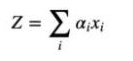
where ai are the individual weights determining attention.
To better understand the concept of attention, let us introduce the following variables – Q, K, V. Q stands for Query which is the context we attempt to look at, Value means the input that is given (either pixels or text features), and Key is the encoded representation of the Value.
For example, in the above image, if :
Query = Green
Key = Building
Then the Value would be,

Hence, to form attention over the input, we need to correlate the query and the key and remove the irrelevant values.
Again consider the example,
| The man was looking at the cloudy sky. (number of words = 8)
Since there are 8 words, we will have 8 queries, 8 keys and 8 values.
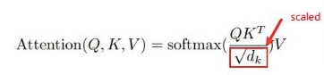
Dimensions of Q = 8X512, for K^T = 512X8, for V = 8X512 and finally for d_k = 512. 512 is the fixed number of dimensions that is fed as input to the encoder.
In the equation, the dot product between the Q and K matrices will result in the concurrent generation of the similarity among them instead of separately computing similarity for each and every word. Moreover, we have a square root of the number of dimensions in the denominator in order to scale the complete value. This will help in ensuring smooth training.
What we understood just now was simple attention, now let’s proceed towards understanding what multi-head attention means?
Multihead attention is a feature used by the transformer which generates h attentions per query instead of one attention. The main reason to use h attention is to obtain h different perspectives for that particular query. Considering so many perspectives will substantially improve the overall accuracy of the model. For the output, all h attentions are concatenated and then fed into the dot product equation.
1.2 Skip Connection and Layer Normalisation:
Another major component of the encoder is the skip connections and the normalisation layers.
Skip connections are basically the residual blocks that connect one layer to another layer by skipping some layers in between. The idea of introducing skip connections was to tackle the Degradation problem (vanishing gradients) in deep neural networks. Skip connections help in optimal training of the network.
The Layer normalization is similar to batch normalization except the fact that in layer normalization, normalization happens across the features in the same layer.
The below image represents the structure of the encoder, displaying the use of multi-head attention, skip connections and layer normalization.
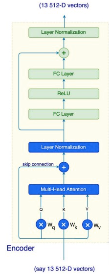
1.3 Feed-Forward Networks:
As demonstrated in the above figure, the output of layer normalization is fed into a fully connected layer, ReLU layer and one more fully connected layer. These operations are applied to each position separately because each output is dependent on the corresponding attention associated with itself.
From the above sections, you have obtained a basic understanding of the different modules present in the encoder and their use.
In the next section, let’s proceed towards understanding the awesome functionalities of BERT.
The BERT Model:
The motivation for using BERT is to address these two major challenges:
- Deep contextual understanding of all the words. Unlike transformers, it attempts to implement a bi-directional word embedding strategy.
- A single model that can serve multiple purposes since training from scratch for every individual task would be computationally expensive as well as time-consuming.
Understanding the Input:
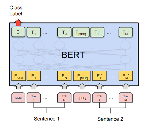
The input comprises sentences splitted into tokens – T1, T2, … Tn. At the beginning, there is always a [CLS] token. If there are multiple sequences in the input then they are splitted by the [SEP] token. The number of output tokens is the same as the number of input tokens. Look at the figure below for better understanding.
The input embeddings comprise of three kinds – Token embeddings, Segment embeddings and Position embeddings.
- Token Embeddings – To compute the embeddings, the input tokens are subjected to transformation to word pieces using an inherent vocabulary (size – 30,000 tokens). For example, the word “bullying” will get splitted into “bully” and “ing”.
- Segment Embeddings – These embeddings ensure the sequence tagging for each token that determines which sequence the token belongs to. In order to do this, the embedding value is added with a constant offset whose value determines the sequence to which it belongs.
- Position Embeddings – This helps to keep track of the positions of the tokens.
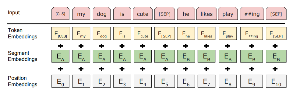
The final embeddings would be the sum of Token embeddings, Segment embeddings and Position Embeddings.
Pre-training and Fine-Tuning Tasks:
The BERT model comprises the two phases – Pre-training and Fine-tuning.
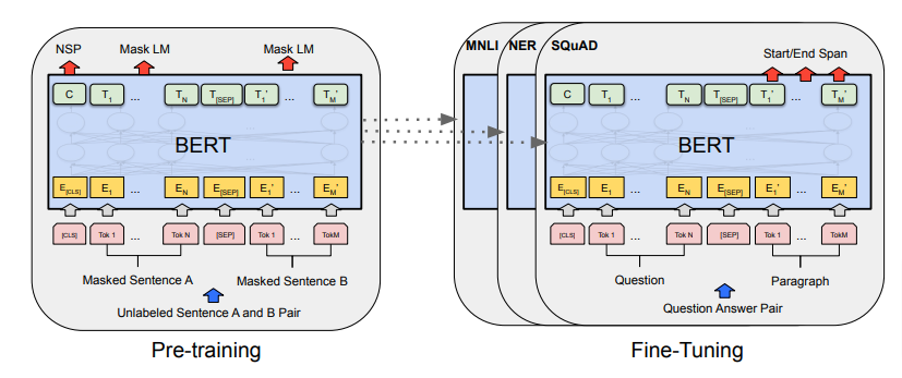
In the pre-training phase, the model is trained with two NLP tasks – (i) Masked Language Model (MLM) and (ii) Next Sentence Prediction (NSP). With the Masked LM, the decoder generates a vector representation of the input which has some masked words.
For example, if the input sentence is – “my cat is furry” then the masked vector would look like – “my cat is [MASK]”.
In this strategy, 80% of the time the word would be masked. 10% of the time, it will be replaced with a random word – “my cat is human”. For the remaining 10% of the time, the word remains unchanged – “my cat is furry”. This learning methodology will make the model robust as it will improve the prediction accuracy. A point to note is that the model won’t be assessed on predicting the whole sequence but only the missing word.
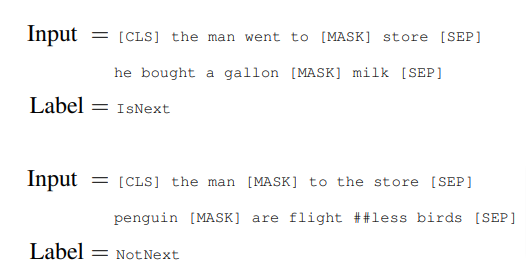
The second NLP task is Next Sentence Prediction (NSP). The input will consist of two sentences – A and B. The idea is to predict whether the second sentence is a follow up of the first sentence or not. This way the model will be able to learn relationships between the two sentences. 50% of the time the model is fed consecutive sentences and the rest 50% sequences are randomly set. Check the figure given below for an example of the NSP task.
To sum up, these two training tasks enable rich learning of contextual information and semantics of the sequences.
The BERT model can be fine-tuned for many different tasks – Natural Language Inference (NLI), Question Answering, Sentiment Analysis, Text Classification and so on. While fine-tuning we keep the complete architecture the same except one last layer which will train the model on custom data. Adding a shallow classifier or a decoder can do the job.
Pretrained Models:
The BERT paper proposed the following pre-trained models:-
- BERT-Base, Uncased: 12-layers, 768-hidden, 12-attention-heads, 110M parameters
- BERT-Large, Uncased: 24-layers, 1024-hidden, 16-attention-heads, 340M parameters
- BERT-Base, Cased: 12-layers, 768-hidden, 12-attention-heads , 110M parameters
- BERT-Large, Cased: 24-layers, 1024-hidden, 16-attention-heads, 340M parameters
Code Implementation:
Now, let’s implement a multi-label text classification model using BERT.
Brief Overview of Multi-Label Text Classification
So, what is multi-label text classification? It is basically the categorization of text into one or more categories to which it belongs. For example, consider the movie review for the film – “Wonder Woman” – “In an entertainment landscape obsessed with flawed heroes, unlikeable heroes and antiheroes, Diana is—unapologetically—a real hero”. From this text it can be predicted that the movie belongs to genres of “fantasy”, “adventure” and “sci-fi”.
Hence, to address a multi-label classification task, the first step is to create the data consisting of cleaned text and one-hot encoded target vector. For example, in the above case, the target vector could look like – [0,0,1,0,1,0,1,0,0…] where 1 represents the categories – fantasy, adventure and sci-fi while 0 represents the remaining absent categories. The second step is to create the word embeddings and finally train the model on those embeddings.
Multi-Label Text Classification with BERT:
Step 1: Installation:
Install the simpletransformers library on google colab using the command: !pip install simpletransformers
Simpletransformers is a library which is built over the famous transformers library – Hugging Face. This makes preprocessing, training and evaluation happen using just a few lines of code.
Step 2: Loading and Preprocessing the data:
We will be working on the kaggle challenge of toxic comment classification wherein the text needs to be classified among the six categories – toxic, severe_toxic, obscene, threat, insult and identity_hate. The dataset can be downloaded from here. Store the downloaded file in your current working directory. We will be using the train.csv file to create both training and evaluation data.
# Import statements

import pandas as pd
from sklearn.model_selection import train_test_split
from simpletransformers.classification import MultiLabelClassificationModel

# ’dir’ would be your current working directory
df = pd.read_csv('dir/train.csv')
# taking nearly 15,000 samples out of nearly 1,50,000 samples
df= df.sample(frac=0.1)

# Combining all the tags into a single list
df['labels'] = df[df.columns[2:]].values.tolist()

# Removing '\n' from the text
df['text'] = df['comment_text'].apply(lambda x: x.replace('\n', ' '))

# Creating new dataframe consisting of just text and their labels
new_df = df[['text', 'labels']].copy()

# Splitting the data into training and testing sets, 80% of data is kept for training and 20% for evaluation
train, eval = train_test_split(new_df, test_size=0.2)
Step 3: Loading the pretrained BERT model:
Here, we will be using the pretrained ‘roberta-base’ version of the roberta model. RoBERTa stands for Robustly Optimised BERT Pretraining Approach. RoBERTa improvises the performance due to the following changes in the original BERT model – longer training, use of more data along with longer training sequences, dynamic masking pattern and removal of next sentence prediction objective from the pretraining task.
'''
Description of params:
model_type: type of the model from the following {'bert', 'xlnet', 'xlm', 'roberta', 'distilbert'}

model_name: choose from a list of current pretrained models {roberta-base, roberta-large} roberta-base consists of 12-layer, 768-hidden, 12-heads, 125M parameters.
num_labels: number of labels(categories) in target values

args: hyperparameters for training. max_seq_length truncates the input text to 512. 512 because that is the standard size accepted as input by the model.
'''
model = MultiLabelClassificationModel('roberta', 'roberta-base', num_labels=6, args={'train_batch_size':2, 'gradient_accumulation_steps':16, 'learning_rate': 3e-5, 'num_train_epochs': 2, 'max_seq_length': 512})
Step 4: Training the model:
# train_model is an inbuilt function which directly trains the data with the specified parameter args. Output_dir is the location for the model weights to be stored in your directory.

model.train_model(train, multi_label=True, output_dir='/dir/Output')
Step 5: Evaluating the model:
'''
Description of params:

result: Label Ranking Average Precision (LRAP) is reported in the form of a dictionary
model_outputs: Returns model predictions in the form of probabilities for each sample in the evaluation set
wrong_predictions: Returns a list for each incorrect prediction

'''

# eval_model is an inbuilt method which performs evaluation on the eval dataframe
result, model_outputs, wrong_predictions = model.eval_model(eval)

# Converting probabilistic scores to binary - 0/1 values using 0.5 as threshold
for i in range(len(model_outputs)):
  for j in range(6):
    if model_outputs[i][j]<0.5:
      model_outputs[i][j] = 0
    else:
      model_outputs[i][j] = 1
Step 6: Prediction:
The test.csv file will also be downloaded in the dataset from here. It contains just the text and does not contain the labels.
# Reading the test data for prediction
test_data = pd.read_csv('dir/test.csv')

# Replacing '\n' values in the text
predict_data = test_data.comment_text.apply(lambda x: x.replace('\n', ' '))

# Convert the dataframe to a list as the predict function accepts a list
predict_data = predict_data.tolist()

# Makes predictions for the test data
predictions, outputs = model.predict(predict_data)
Conclusion:
In this article, we explored the BERT model in depth. We also developed a basic understanding of the encoder module used from the transformer. The BERT model proves to be an edge over other previous models due to its property of Bidirectional Encoding. This model is pre-trained and can be fine-tuned for several tasks such as Natural Language Inference (NLI), Sentiment Analysis, Multiclass/Multilabel text classification and many more. The model has definitely improved the accuracy in several fields by severely cutting down the requirement of training from scratch of different models for different purposes.