Introduction
Humans have the ability to understand words and derive meaning from them easily. In today’s world, however, most of the tasks are performed by computers. For example, if you want to know whether it is going to be sunny or rainy today, then you will have to type a text query in Google. Now, the question is how will a machine understand and process such a huge amount of information presented in the text on such a frequent basis? The answer to that is word embeddings.
Word Embeddings are basically vectors (text converted to numbers) that capture the meanings, various contexts, and semantic relationships of words. An embedding is essentially a mapping of a word to its corresponding vector using a predefined dictionary.
For instance,
Sentence: It will rain heavily today.
Dictionary: {“It”: [1,0,0,0,0], “will”: [0,1,0,0,0], “rain”: [0,0,1,0,0], “heavily”: [0,0,0,1,0], “today”: [0,0,0,0,1]}
Here, every word has been assigned a unique vector (for example) in order to differentiate all of them.
Types of word embeddings:
1. Count Vector:
Let’s consider a number of documents {d1, d2, …, dn} which consist of any arbitrary text information. Consider N as the number of unique tokens extracted from a corpus C taken from the given data.
In order to create a count matrix M of dimensions CXN, frequency of each of the unique words needs to be obtained for every document belonging to corpus C.
For example,
Let the corpus comprise three sentences.
S1 = In monsoon, it will rain.
S2 = rain rain come again.
S3 = sun is visible in summer. In the monsoon, the sun is hidden by clouds.
Let N be the list of unique words = [‘monsoon’, ‘rain’, ‘come’, ‘again’, ‘sun’, ‘visible’, ‘summer’, ‘hidden’, ‘clouds’]
Dimensions of the count matrix will be 3X9 as there are three documents in the corpus and nine unique words.
The count matrix is demonstrated as below:
| monsoon | rain | come | again | sun | visible | summer | hidden | clouds | |
| S1 | 1 | 1 | 0 | 0 | 0 | 0 | 0 | 0 | 0 |
| S2 | 0 | 2 | 1 | 1 | 0 | 0 | 0 | 0 | 0 |
| S3 | 1 | 0 | 0 | 0 | 2 | 1 | 1 | 1 | 1 |
Advantages:
- Less computationally expensive as only the frequency of the word is to be considered.
Disadvantages:
- Since the calculation is just based on count and there is no consideration for the context of a word, the method proves to be less beneficial.
Code:
#Importing libraries
from sklearn.feature_extraction.text import CountVectorizer
import nltk
from nltk.corpus import stopwords
from nltk.tokenize import word_tokenize

#Downloading stopwords and punkt packages
nltk.download('stopwords')
nltk.download('punkt')

#Initialising stopwords for english
set(stopwords.words('english'))

#sample sentences
text = ["In monsoon, it will rain", "rain rain come again", "sun is visible in summer. In the monsoon, the sun is hidden by clouds"]

#set of stop words
stop_words = set(stopwords.words('english'))
all_sentences = []

#Logic for removing stop words and obtaining filtered sentences from the list

for i in range(len(text)):
  word_tokens[i] = word_tokenize(text[i])
  tokenized_sentence = []

  for j in word_tokens[i]:
      if j not in stop_words:
          tokenized_sentence.append(j)
  all_sentences.append(" ".join(tokenized_sentence))

#Initialising the CountVectorizer
countvectorizer = CountVectorizer()

#Applying CountVectorizer to the list of sentences
X = countvectorizer.fit_transform(all_sentences)

#Converting output to array
result = X.toarray()

print("Sentences after removing stop words", all_sentences)
print("Count Vector:", result)
2. TF-IDF:
TF-IDF stands for Term Frequency-Inverse Document Frequency. This method is an improvisation over the Count Vector method as the frequency of a particular word is considered across the whole corpus and not just a single document. The main idea is to give more weight to the words which are very specific to certain documents whereas to give less weight to the words which are more general and occur across most documents.
For example, general words such as “is”, “the”, “and” would be frequently occurring while words such as “Donald Trump” or “Indira Gandhi” would be specific to a particular document.
Mathematically,
Term Frequency (TF) = Number of times a term appears in a document / Total number of terms in the document
Inverse Document Frequency (IDF) = log(N/n) where N is the total number of documents and n is the number of documents a term has appeared in.
Consider the following example.
Given are two documents – D1 and D2.
|
Document 1 |
Document 2 |
| Term Count | Term Count |
| Today 1 | Today 1 |
| is 3 | is 3 |
| sunny 4 | rainy 5 |
| day 2 | day 1 |
TF(Today, Document 1) = 1/8
TF(Today, Document 2) = 1/8
TF(sunny, Document 1) = 4/8
IDF(Today) = log(2/2) = log(1) = 0
IDF(sunny) = log(2/1) = log(2) = 0.301
Therefore,
TF-IDF(Today, Document 1) = 1/8 * 0 = 0
TF-IDF(Today, Document 2) = 1/8 * 0 = 0
TF-IDF(sunny, Document 1) = 4/8 * 0.301 = 0.1505
From the above calculations, it can be seen that the common word “Today” has lower weight as compared to the word “sunny” which is an important word for the context of Document 1.
Advantages:
- It is computationally easy.
- Most essential words of a document are extracted with a basic calculation and do not involve many efforts.
Disadvantages:
- It cannot capture the semantics of a word, works only like a lexical-level feature.
Code:
from sklearn.feature_extraction.text import TfidfVectorizer
import pandas as pd

#Declaring the list of sentences
documents = ['Today is sunny day', 'Today is rainy day']

#Initialising Tfidf Vectorizer
vectorizer = TfidfVectorizer()

#Fitting the Vectorizer to the list
X = vectorizer.fit_transform(documents)
print(X)

#Printing the feature names
print(vectorizer.get_feature_names())

matrix = X.todense()
tfidf_list = matrix.tolist()
tfidf_df = pd.DataFrame(tfidf_list, columns = vectorizer.get_feature_names())

print(tfidf_df)
3. Word2Vec:
Word2Vec is a prediction-based method for forming word embeddings. It is a shallow two-layered neural network that is able to predict semantics and similarities between the words, unlike the deterministic methods. Word2Vec is a combination of two different models – (i) CBOW (Continuous Bag of Words) and (ii) Skip-gram.
Overview of the models – CBOW (Continuous Bag of Words) and Skip-gram.
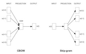
3.1 CBOW (Continuous Bag of Words):
This model is a shallow neural network that predicts the probability of a word given a certain context. Here, the context refers to the input of words surrounding the word to be predicted.
The architecture of CBOW model:
- As a first step, the input is created by forming a bag of words for the given text.
For example,
Sentence 1 = All work and no play make Jack a dull boy.
Sentence 2 = Jack and Jill went up the hill.
Bag of Words: {“All”:1, “work”:1, “no”:1, “play”:1, “makes”:1, “Jack”:2, “dull”:1, “boy”:1, “Jill”:1, “went”:1, “up”:1, “hill”:1} (after removing the stop words)
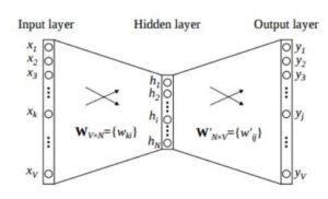
This input consisting of words and their frequency of occurrence is sent as a vector to the input layer. For X number of words, input would be X[1XV] vectors, where V is the maximum length of the vector.
- Next, the input-hidden layer matrix consists of dimensions VXN, where N is the number of dimensions the word is represented in. The output-hidden layer matrix consists of dimensions NXV. Here, the values are calculated by multiplying the input to hidden input weights.
- In the output layer, the output is calculated by multiplying hidden input to the hidden output weights. The weight calculated between the hidden layer and the output layer gives the word representation. As a continuous intermediate step, the weights are adjusted by using backpropagation over the error calculated between the output and the target values.
Advantages:
- The method being probabilistic gives better results as opposed to the deterministic methods.
- The memory requirement is less as huge matrices don’t need to be calculated.
Disadvantages:
- Optimization is extremely important when otherwise, the training will take long hours to complete.
3.2 Skip-gram:
The Skip-gram model predicts the context given a word, just opposite to what CBOW does.The architecture of the Skip-gram model:
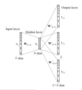
Input layer size: [1XV], Input hidden weight matrix size: [VXN], Output hidden weight matrix: [NXV], Output layer size: C[1XV]
The input to the model and further steps till the hidden layer would be similar to CBOW. The number of output target variables would be dependent on the size of the context window. For example, if the size of the context window is 2 then there will be four target variables, two words before the given word and two after.
Four separate errors would be calculated with respect to the four target variables and the final vector is obtained by performing element wise addition. This final vector is then backpropagated to update the weights. For training, the weights between the input and the hidden layer are used for word representation.
Advantages:
- Skip-gram model can capture different contextual information for a word as there would be different vector representations for every context.
- More accurate for infrequent terms and works well for larger databases.
Disadvantages:
- It requires more RAM for processing.
Code:
To use pre-trained Word2Vec model from genism library:
import gensim
import gensim.downloader as api
from gensim.models.keyedvectors import KeyedVectors

#loading pretrained model
nlp_w2v = api.load("word2vec-google-news-300")

#save the Word2Vec model
nlp_w2v.wv.save_word2vec_format('model.bin', binary=True)

#load the Word2Vec model
model = KeyedVectors.load_word2vec_format('model.bin', binary=True)

#Printing the most similar words to New York from vocabulary of pretrained model
model.most_similar('New_York')
To train the Word2Vec model from scratch:
import gensim
'''
Data for training Word2Vec
train: A data frame comprising of text samples
'''

#training data
corpus = train

#creates a list for a list of words for every training sample
w2v_corpus = []
for document in corpus:
   w2v_words = document.split()
   w2v_grams = [" ".join(w2v_words[i:i+1])
               for i in range(0, len(w2v_words), 1)]
   w2v_corpus.append(w2v_grams)

#initialising and training the custom Word2Vec model
'''
size: dimensions of word embeddings
window: context window for words
min_count: words which appear less number of times than this count will be ignored
sg: To choose skip-gram model
iter: Number of epochs for training
'''

word2vec_model = gensim.models.word2vec.Word2Vec(w2v_corpus, size=300,
            window=8, min_count=1, sg=1, iter=30)

#vector size of the model
print(word2vec_model.vector_size)

#vocabulary contained by the model
print(len(word2vec_model.wv.vocab))
4. GloVe:
GloVe stands for Global Vectors for Word Representation. This algorithm is an improvement over the Word2Vec approach as it considers global statistics instead of local statistics. Here, global statistics mean, the words considered from across the whole corpus. GloVe basically attempts to explain how frequently a particular pair of words occur in a document. For this, a co-occurrence matrix is constructed which will represent the presence of a particular word relative to the other word.
For example,
Corpus – It is rainy today, tomorrow it will be sunny and the day after will be windy.
|
rainy |
today |
tomorrow |
sunny |
day |
after |
windy |
|
|
rainy |
0 |
1 |
0 |
0 |
0 |
0 |
0 |
|
today |
1 |
0 |
0 |
0 |
0 |
0 |
0 |
|
tomorrow |
0 |
0 |
0 |
0 |
0 |
0 |
0 |
|
sunny |
0 |
0 |
0 |
0 |
0 |
0 |
0 |
|
day |
0 |
0 |
0 |
0 |
0 |
1 |
0 |
|
after |
0 |
0 |
0 |
0 |
1 |
0 |
0 |
|
windy |
0 |
0 |
0 |
0 |
0 |
0 |
0 |
The above matrix represents a co-occurrence matrix whose values denote the count of each pair of words occurring together in the given example corpus.
After computing the probability of occurrence for the word “rainy” given “today”, p(rainy/today) and “rainy” given “tomorrow”, p(rainy/tomorrow), it turns out that the most relevant word to “rainy” is “today” as compared to “tomorrow”.
Code:
#Import statements
from numpy import array
from numpy import asarray
from numpy import zeros
from keras.preprocessing.text import Tokenizer

#Download the pretrained GloVe data files
!wget http://nlp.stanford.edu/data/glove.6B.zip

#Unzipping the zipped folder
!unzip glove*.zip

#Initialising a tokenizer and fitting it on the training dataset
'''
train: a dataframe comprising of rows containing text data
'''
tokenizer = Tokenizer(num_words=5000)
tokenizer.fit_on_texts(train)

#Creating a dictionary to store the embeddings
embeddings_dictionary = dict()

#Opening GloVe file
glove_file = open('glove.6B.50d.txt', encoding="utf8")

#Filling the dictionary of embeddings by reading data from the GloVe file
for line in glove_file:
    records = line.split()
    word = records[0]
    vector_dimensions = asarray(records[1:], dtype='float32')
    embeddings_dictionary[word] = vector_dimensions
glove_file.close()

#Parsing through all the words in the input dataset and fetching their corresponding vectors from the dictionary and storing them in a matrix
embedding_matrix = zeros((vocab_size, 50))
for word, index in tokenizer.word_index.items():
    embedding_vector = embeddings_dictionary.get(word)
    if embedding_vector is not None:
        embedding_matrix[index] = embedding_vector

#Displaying embedding matrix
print(embedding_matrix)
Conclusion:
In this blog, we reviewed a number of methods – Count Vector, TF-IDF, Word2Vec, and GloVe, for creating word embeddings from the raw text data. It is always a good practice to preprocess the text and then send the preprocessed data for creating the word embeddings. As a further step, these word embeddings can be sent to machine learning or deep learning models for various tasks such as text classification or machine translation.